
After nearly 30 years working with Excel across companies in different industries, I keep seeing the same scene over and over: capable analysts and administrators wasting valuable time with VLOOKUPs that break, helper columns that no one understands, and files that only one person knows how to maintain.
That real pain —and the certainty that there had to be a much better way— was exactly what led me to design and build Optipe’s applications.
Today, merging tables with one, two, or even three criteria is something anyone on your team can do in seconds, without writing a single formula and with stable results.
Imagine this: You have one table with sales by product code and another with product names, prices, stock, and suppliers. You need to bring all the complementary information, audit missing codes, or sum sales by category. This is a task that most Excel users perform daily.
Keep struggling with complicated formulas? ❌
Or automate table merging in seconds? ✅
📊 The Main Classic Ways to Merge Tables
1. VLOOKUP
The most well-known function for years. It searches in the first column and returns a value from the same row.
Advantages: Very simple for quick and basic merges.
Limitations: Only searches to the right, does not easily support multiple criteria, and breaks if columns are inserted or moved. It is fragile and error-prone.
2. XLOOKUP
The modern successor to VLOOKUP (available in Excel 365 and 2021). It can search in any direction and return values to the left.
Advantages: More flexible, better error handling, and can search from the end.
Limitation: Not available in older versions of Excel.
3. Helper Column
A very common technique when you need to merge by more than one criterion (e.g., Branch + Product Code). A combined key is created in both tables.
Advantage: Allows using VLOOKUP with multiple conditions.
Major disadvantage: It modifies the original data, complicates the file, and any change requires recalculating everything.
4. INDEX + MATCH
The most flexible combination. It allows lookups in any direction and with multiple criteria without a helper column.
Advantage: Very powerful and efficient in large files.
Disadvantage: Complex syntax that is hard to remember and prone to errors.
5. SUMIF / COUNTIF and .IFS
Ideal functions for summing or counting values that meet one or multiple criteria in another table.
Advantage: Very useful for quick audits and summary reports (e.g., “Does this code exist?”).
Limitation: Syntax becomes complicated when there are many criteria.
6. Conditional Statistics (MAXIFS, MINIFS, AVERAGEIFS)
Find the maximum, minimum, or average value based on specific conditions.
Advantage: Excellent for analysis and dashboards.
Limitation: Requires newer versions of Excel and the syntax is not always intuitive.
Excel Functions Commonly Used to Cross-Reference Tables
- VLOOKUP
- XLOOKUP
- INDEX + MATCH
- SUMIFS
- COUNTIFS
- MAXIFS
- MINIFS
⚡ The Ultimate Solution: Merge Tables in Data Tools Suite
All the previous techniques require writing complex formulas, creating helper columns, and debugging errors repeatedly. Merge Tables from Data Tools Suite eliminates that complexity completely:
- Merge up to 3 criteria without helper columns
- Multiple merge types: lookup, sum, count, position, compare lists, average, max, min, and more
- Returns results as static values or as formulas (the tool writes perfect formulas for you)
- Clear visual indicator of matches and non-matches
- Massive time savings on repetitive tasks
In practice: select the tables, choose the type of merge, and the tool automatically generates the result in seconds.
Also related: The Create Conditional Formula tool lets you enter any complex formula in a guided way without errors. See Create Conditional Formula →
Also check out the Compare Lists app to quickly see which values match or which ones are missing from your table. View Compare Lists →
Practical Example: Cross-referencing two tables in Excel by 2 conditions
💡 Example: Table Cross-Reference by 2 criteria (City and Department)
Imagine you need to consolidate the Salesperson name and total Sales into your main list ("City-Dpmnt") from a separate, detailed report ("Sales"). Instead of struggling to build complex array formulas to evaluate both conditions simultaneously, the tool automates this entire process instantly.
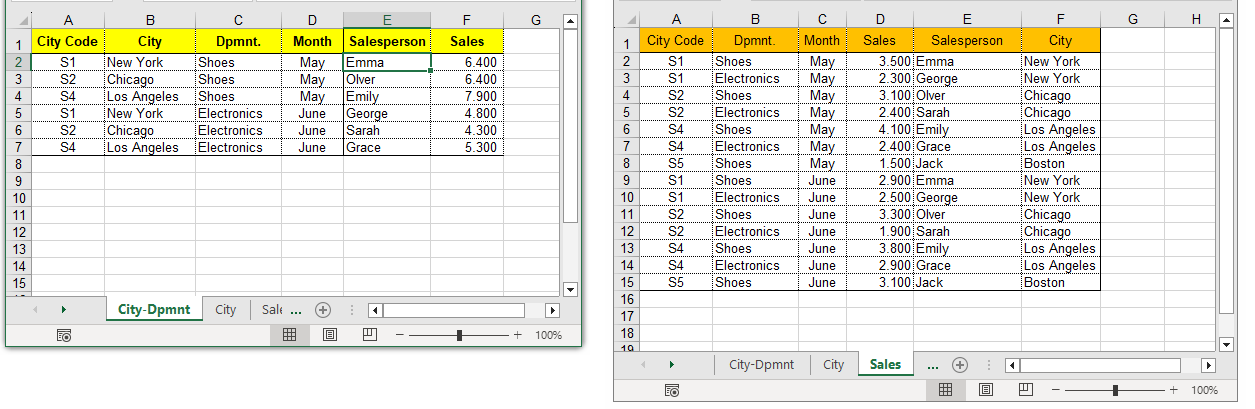 Cross-referencing data by combining City and Department criteria at the same time.
1. Find the Salesperson name in Table2:
Retrieves the exact text from the Salesperson column by matching the City ($B2) and Department ($C2) criteria simultaneously.
2. Sum the Total Sales from Table2:
Aggregates the numeric values from the Sales column that meet both the specified City and Department parameters.
🚀 The automation secret: Manually writing an INDEX formula with multi-criteria conditions requires advanced knowledge of array structures in Excel, flawless cell anchoring, and is highly prone to typos. With OPTIPE's Cross-Reference Tables feature, you simply map the matching columns through an intuitive visual wizard, and the add-in writes and extends perfect formulas for you in a split second.
⏱️ Manual vs Automated: Real Time Savings
| Task | Manual Formulas | Merge Tables |
|---|---|---|
| Simple merge (1 criterion) | 5-15 minutes | 20 seconds |
| Multiple criteria merge | 30-60 minutes | 1 minute |
| WEEKLY TOTAL | 3-6 hours | 10 minutes |
📚 Recommended Resources on Merging Tables
📚 Want to keep improving your Excel productivity?
Go to Optipe Blog →💡 Create Advanced Lookup, Sum and Count Formulas in Excel Automatically
Increase your productivity in Excel and save hours every week
Forget complex formulas and calculations. Automate your work with Data Tools Suite and MultiMail.
Try it. You'll get it.
🎯 Download Free Now!")
")
")
")